CMCF - Data Collection Primer

Data Collection

The following sections are meant to provide practical advice on data collection on protein crystals at CMCF for those with experience collecting diffraction data. If you are new to collecting X-ray diffraction data, we advise working with your supervisor or experienced mentor until familiar with the process.

Native Datasets

Native datasets are used to obtain high-resolution data in order to discern as much detail as possible about a structure or ligand. They are also used to solve new structures using Molecular Replacement methods when a similar structure is available. Therefore, obtaining the highest resolution spots is the primary motivation. However, it is also important to minimize overloaded pixels in the lower resolution spots for successful molecular replacement, as well as minimize radiation damage for a complete high-quality dataset.

To accomplish these goals, the collection parameters must be carefully balanced. Detector distance is adjusted such that all the desired spots fall on the detector surface with maximal spot separation. A rotation angle per frame, along with start and total angles must be selected to minimize overlaps while maintaining a reasonable total time for data collection. In general, a sufficient total angle should be collected to achieve a multiplicity in the dataset of 4 or more whenever possible (above 1 in the case of P1). Finally, an exposure is chosen to obtain maximum intensity, balanced with the need of minimizing radiation damage which will decrease the quality of the dataset.

Wavelength/Energy. The exact energy setting used for collecting native datasets is not critical, but is generally chosen such that it lies within the higher flux region specific to the beamline. Depending on the beamline mode, you may be able to change the energy to capture anomalous data to allow for phasing by common elements such as sulfur or selenium.

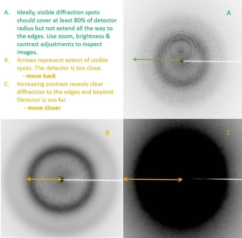
Detector Distance. During the initial screening, take note of the quality of diffraction, and how well the crystal diffraction fills the image. Use the zoom feature, brightness & contrast settings to inspect the image. The middle mouse wheel can be conveniently used to adjust the image brightness to visualize how far the spots extend from the centre of the image. You may not see the weakest spots if the image is too bright; darkening the image and zooming into the areas farther from the centre allows you to inspect these spots. Shorter detector distances result in higher resolution at the edges. Note there are detector distance limits built into the data collection software.

Guideline: detector distance should be adjusted so that visible spots extend to cover approximately 80% of the distance from the centre of image to edge of the detector. The faintest spots may not be visible to the eye but may still be present some distance from the visible ones. When in doubt, the Auto.process screening report provides an appropriate estimate of the resolution limit.

Rotation Angle Per Frame, Starting & Total Angle Range. The Autoprocess algorithm is run with each sample screen that has 3 or more images and the results can be viewed in the analysis window of MxDC. You may also run Autoprocess or other programs such as Mosflm manually in order to get an idea of your unit cell, symmetry parameters and obtain recommendations for rotation angle per frame (delta angle), total angle range, and the best starting angle. In general, smaller rotation angles per frame are used for larger unit cells. Larger total angles are generally needed for lower symmetry crystals.

Optimize the rotation angle/frame, start angle and total angle according to the Autoprocess recommendations. A rotation angle per frame around 0.2 degrees is usually reasonable (0.5 to 1 degree for screening). For large unit cells, 0.1 or 0.15 degrees may provide better results. When considering the total angle, aim for multiplicity of 4 or higher (above 1 in the case of P1). If there is uncertainty, a total angle of 180 degrees is usually sufficient.

Exposure. The MxDC software offers powerful options for optimizing the experiment. Beneath the diffraction image pane is an Information Button. The information window can be kept open during data collection and displays information about each image.

CMCF-BM Guidelines (PILATUS detector): Generally expect an average intensity between about 10 and 30. On beamline CMCF-BM using the high flux (DMM) mode, typical exposure is 0.2 seconds / 0.2 degrees. The time should be chosen to be roughly equivalent to the angle per frame (for example 0.1 - 0.2 seconds / 0.1 degrees). Higher exposure time / angle increment will result in increasing radiation damage to the sample with minimal resolution gains. When using normal flux (DCM) beam, typical exposure is 0.4 - 2 seconds / 0.2 degrees. The beam size is adjustable between 20 - 200 microns; keep in mind that there will be lower flux on the sample with smaller beam sizes.

CMCF-ID Guidelines (EIGER detector): Generally expect an average intensity between about 2-10, and ideally below 5. On beamline CMCF-ID in DCM mode, typical exposure is 0.02 seconds / 0.2 degrees. The time should be chosen to be roughly 1/10 of the angle per frame (for example 0.005 - 0.015 seconds / 0.1 degrees). Higher exposure time / angle increment will result in increasing radiation damage to the sample with minimal resolution gains. The beam size is adjustable between 5 - 50 microns; the flux decreases approximately linearly with beam size (i.e. a 50 um beam is approximately 10-fold stronger than the 5 um beam)..

Recommended Reading

SAD Datasets

Single-wavelength Anomalous Diffraction (SAD) datasets are used to identify heavy-atom positions and/or solve new structures for which a suitable Molecular Replacement model is unavailable. Data are generally collected at the peak of the absorption curve of a naturally-occuring heavy atom or heavy atom derivative. Very accurate measurement of the lower-resolution data is important in order to measure anomalous intensity differences. To accomplish this, radiation damage must be minimized and good quality high multiplicity data obtained.

Planning. Both CMCF beamlines can be used to collect anomalous datasets, but in general, the CMCF-BM beamline is chosen. It is more intuitive to avoid over-exposure and radiation damage on this beamline, while still obtaining sufficient intensities for SAD phasing. Before starting, be familiar with the heavy atom being used and its energy absorption edges. This information can be found on X-ray Absorption Edge Tables, and on the Scans page of MxDC. The CMCF beamlines can generally reach energies between 6 - 18 keV. For energies below this, the absorption edge cannot be reached and Sulfur-SAD (S-SAD) methods should be used instead.

Wavelength/Energy. Check the X-ray Absorption Edge Tables to choose an appropriate accessible energy for your heavy atom derivative (between 6 - 18 keV), or examine the periodic table display on the Scans page of MxDC. Adjust the beamline energy to a value near the edge of interest and, in the case of CMCF-ID, optimize the beam before continuing.

Before starting the MAD Scan, make sure your sample is centred properly. It is a good time to take the diffraction screening images to ensure the crystal is centred, to check the quality of diffraction, and to also get the Autoprocess screening algorithm started. Remember to use the "anomalous" option in Autoprocess or Mosflm to obtain an appropriate data collection strategy.

From the Scans page in MxDC, perform a MAD Scan. The following is an example of a scan obtained from a Zn-containing sample.

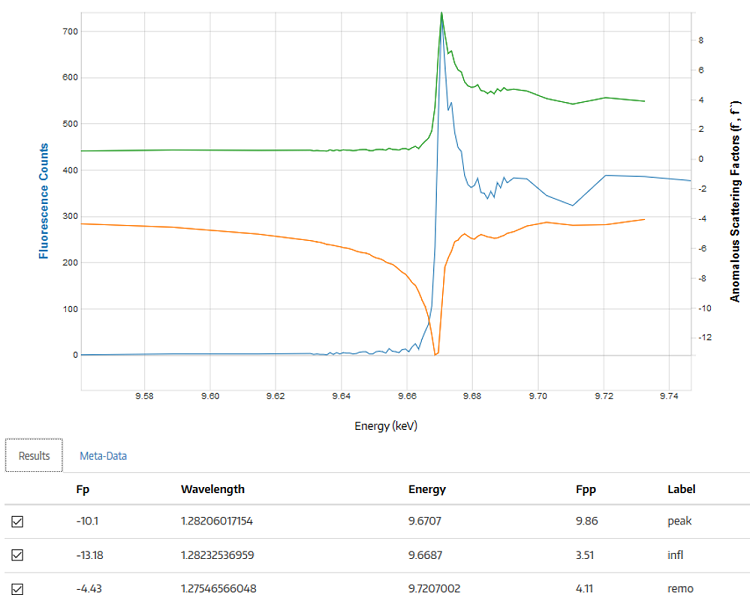
Along the x-axis, the energy is displayed in units of keV. The y-axis represents fluorescence counts. The fluorescence detector will saturate around 15,000 counts so attenuation is needed if the readings are too high. If the result is a flat line at 0 counts, check that there is appropriately optimized beam, that the beamline shutters are open and that your sample is centred properly. If there is still no reading, call your user support person for help. If there is no metal in the sample, you will get a low level reading that is essentially noise with no distinct peak. Exposure can be increased (and/or attenuation decreased) to ensure fluorescent count levels of around 50 - 100. This is a good starting base level for MAD Scans in general.

Note: An XRF Scan (Excitation Scan) can be used instead of a MAD Scan to identify metals in the sample if there is uncertainty. To perform an Excitation Scan, the beamline energy must be optimized above the absorption edge(s) of the atom(s) of interest, instead of near the absorption edge. Be aware that other elements near the sample may sometimes also be detected, such as from the beamstop or the sample pin. In addition to an excitation scan of your sample, it is recommended you take a blank excitation scan with no sample in the beam in order to detect other elements near the sample position that are not part of your sample of interest.

Once the MAD Scan is complete, Chooch will automatically be run and the peak energy output, along with inflection energy and a suggested remote energy. Inflection & remote energies would be used in addition to the peak energy for a Multiple-wavelength Anomalous Diffraction (MAD) experiment if desired. The calculated peak energy should correspond to the peak energy visible in the plot, and is the energy used for SAD data collection.

Adjust the beamline to the peak energy and, in the case of CMCF-ID, optimize. In the Data page of MxDC, make sure the peak energy and other values are correctly defined before starting the collection.

Detector Distance. In general, detector distance can be chosen as for native datasets, described above.

Rotation Angle Per Frame, Starting & Total Angles. When the Autoprocess screening algorithm is run with the anomalous mode enabled, suggested values will be provided for collecting anomalous data. Mosflm has a similar anomalous option. An important difference for setting these values, as compared with native data, is the total angle.

Guideline: Larger total angle is needed for more multiplicity; 360 degrees is not uncommon. The amount of data collected may be judged by the anomalous signal obtained after collecting some images and/or solving the metal sites. Autoprocess in anomalous mode provides "anomalous signal" and "anomalous correlation" values. Look for anomalous signal at least above ~1 in low resolution shells, with significant correlation. The higher the better. At some point, radiation damage will outweigh the benefit of collecting more frames. In some cases, combining data from multiple crystals may be necessary.

Exposure. This should be much less than for native datasets. Radiation damage must be minimized as much as possible, therefore:

CMCF-BM Guideline (PILATUS detector): 0.2 seconds or more should be used to keep detector readout error <1%; beam attenuation may be required to minimize radiation damage.

Recommended Reading

S-SAD Datasets

A Sulfur-SAD (S-SAD) experiment is a special case of SAD experiment in which anomalously-scattering sulfur atoms, naturally present in most proteins, are used to solve the structure. In this case, the absorption edge (sulfur K edge = 2.47 keV) is beyond the lower energy limit of a typical crystallography beamline, including CMCF beamlines. Similar methods can be used for iodine (L1 edge 5.19 keV), cesium (L1 edge 5.71 keV), and several other elements which also have absorption edges near the lower accessible limit or below, with no edges within the optimal beamline energy range.

Since the absorption edge is below the energy range of the beamlines, a MAD Scan is not performed. Instead, the energy is optimized near the lower limit of the beamline (usually between 6.0 – 7.0 keV), where some anomalous scattering can still be observed. Since the signal is weaker farther from the absorption edge, and air scattering becomes more prominent at lower energies, care must be taken to measure the reflections accurately.

Planning. Both CMCF beamlines can be used to collect S-SAD datasets, but in general, the CMCF-BM beamline is chosen. It is more intuitive to avoid over-exposure and radiation damage on this beamline, while still obtaining sufficient intensities for S-SAD phasing.

Wavelength/Energy. The recommended energy is 7.0 keV.

Detector Distance. In general, the diffraction pattern should be of high quality with well-separated spots. The detector distance should be somewhat closer than for experiments using higher energies because the effects of air scattering become more prominent at lower energies.

Rotation Angle Per Frame, Starting & Total Angles. These can be chosen in a similar manner as for SAD experiments, described above. However, typically more data are needed for S-SAD.

Guideline: Larger total angles are needed for more multiplicity but this has to be balanced carefully with minimizing radiation damage. One or more 360 degree passes are not uncommon. The detector distance (and/or Chi angle on CMCF-BM) can be adjusted slightly for different passes so that diffraction spots are measured on different parts of the detector with different 360 degree passes. Multiple crystals can be used if radiation damage becomes an issue, and the datasets combined. The amount of data collected may be judged by the anomalous signal and/or solving the sulfur sites. Autoprocess in anomalous mode provides "anomalous signal" and "anomalous correlation" values. Look for anomalous signal above about 1 in low resolution shells, with significant correlation.

Exposure. This should be much less than for native datasets. Radiation damage must be minimized as much as possible.

CMCF-BM Guideline (PILATUS detector): 0.2 seconds or more should be used to keep detector readout error <1%; beam attenuation may be required to minimize radiation damage.

Recommended reading

Data Collection

Native Datasets

SAD Datasets

S-SAD Datasets

Beamline Responsible:

Mailing Address:

Mailing Address: